| Probability. By definition a probability is a ratio of the favorable values of a variable to all the possible values of that variable. In general it is possible to estimate probabilities by measuring the relative frequency of the values of the variable in a sufficiently representative sample. |

| Two basic relationships between attributes. Looking at a record comparison is like observing the results of an experiment that has two or three stages. There are three determinations: 1) is the record comparison matched or not; 2) is there agreement in the data values of each field; 3) is there data present in each field or not? There are two situations that can hold between the attributes we observe, i.e., the stages of an experiment. |
| 1) The second stage may depend on the first stage. For example, first look at a field in a record comparison to see if there is data present in both records. If so, check whether they agree or not. Otherwise, count the pair as having data missing. Agreement or disagreement depends on whether there is data present. | ||
| 2) The second stage may not depend on the first stage. For example, first look at a record comparison and determine whether the records represent the same entity. Whether it does or not, check to see if the data is present in some particular field. Presence of data in a field does not depend on whether the records in the comparison represent the same entity. |
| For the first type of relationship we need the idea of conditional probability, and for the second we need the idea of independent events. |
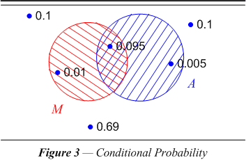
| Example of conditional probability. Conditional probability is denoted by P( A | M ), and reads, “The probability of A, given that M,” or in our case, “The probability that a comparison agrees in some field’s data value (A), provided that it represents a matched pair (M).” To understand the formula for conditional probability consider the universe of six points in figure 3. |

| Each point represents a number of observations of the same kind so that we estimate its probability as indicated. For example, 69% of our comparisons are for unmatched pairs and both fields being compared are blank, 10% of them have the field blank in one record and 10% have the field blank in the other record. We observe also that the data values agree in unmatched comparisons in 0.5% of the cases we look at, and that in matched comparisons it agrees in 9.5% of the cases. The final class of observations are the 1% where the data values in the field in question fail to agree but the agreement in other fields tell us that the comparison clearly represents a matched pair. The total probability in this universe is 100% of our observations. |
| Calculating conditional probabilities. To assign P( A | M ) a value we must consider M as the new universe. Within that new universe we see just one A outcome, with a probability of 0.095. But a probability of 0.095 (with respect to the old universe where the total probability is one) counts for more in this new M universe, which has a total probability of 0.105. It seems natural to choose P(A | M ) = 0.095 ÷ 0.105, i.e., 0.905. The idea in general is |

| This is the inclusion of one set in another, but we may also rewrite this equation as a rule for the intersection of multiple sets in general, i,e., the logical AND: |
| P(Ai and M) = P(M) × P(Ai | M). |
| (NB: We use the subscript on A to specify which field the agreement probability refers to.) The AND rule says that if M occurs 10.5% of the time and Ai occurs 90.5% of those times, then Ai and M occur simultaneously 9.5% of the time. Because AND is symmetrical we can also conclude that |
| P(Ai and M) = P(Ai) × P(M | Ai) |
| Independence of events. If two events are unrelated so that the occurrence (or non-occurrence) of one of the events doesn't affect the likelihood of the other event, the events are called independent. We say that two events are independent if and only if (iff) |
| P(Pi and M) = P(Pi) × P(M) |
| To see why this reflects our intuition about independence, combine this with the rules for AND, i.e., being matched (M) has no effect on whether data is present in the field (Pi), or symmetrically, Pi has no effect on M. |
| iff P(M) = P(M | Pi) or iff P(Pi) = P(Pi | M) |
| This means that when the data values in the fields of a record are independent, their combined probability is the product of their individual probabilities. |
| P(A1 and A2 and A3 and . . . ) = P(A1) × P( A2) × P( A3) × . . . |
| The theorem of total probability. These last few paragraphs are about multi-stage experiments. Typically the investigator does not know the first stage. The stage that is hidden to us is whether the comparison is matched. However, the investigator is able to measure the results of the subsequent stages. The stages that we can observe and measure are 2) whether there is data present in the fields of the records being compared, and 3) whether the data values in the corresponding fields of the record comparison agree or not. |
| We simplify the situation to two stages to introduce the theorem of total probability. In terms of just four outcomes, we have: matched (M) or unmatched (¬M), and data agreement in field i (Ai) or not agreeing in the field (¬Ai). If at the first stage the result is exactly one of either M or ¬M, then the probability of Ai at the second stage is |
| P(Ai) = P(M) × P(Ai | M) + P( ¬M) × P(Ai | ¬M) |

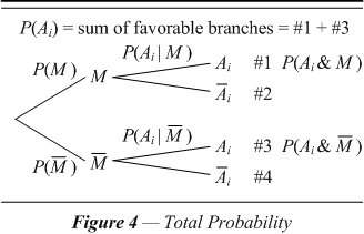
| The student may find it easier to apply the theorem of total probability by referring to the various branches of a diagram such as the one in figure 4. Each branch represents the product of two probabilities. You simply add up the favorable branches — those that lead to the desired attribute. |
| Bayes’ theorem. Bayes’ theorem is a way of allowing conditional probability to look backward. It states that the a posteriori of M at the first stage, i.e., as a hidden probability — an explanatory variable — given Ai on the second stage is P(M | Ai ) = P(Ai and M) ÷ P(Ai), which being interpreted according to the diagram in figure 4 is |

| Suppose we have a sample of records and that 0.5% of all the record comparisons we can possibly make are matched M. This is a way of looking at the duplication rate. Suppose further that we choose agreement in a particular field as the response variable and that in observing the values in the matched record pairs, we find that some of them, say 2% of the pairs actually disagree in that field. We say that the reliability of the field is 98%. Moreover, suppose that in looking at all the comparisons we note that among those that agree 3% are not matched pairs; the data values in the field agree by coincidence. What if in a particular pair the field agrees? To what degree is it safe to conclude that the comparison is matched? Assigning the probabilities to the branches in figure 4 we find that the total probability of agreement is: |
| P(Ai) = #1 + #3 = (0.005) × (0.98) + (0.995) × (0.03) = 0.035 |
| By Bayes’ theorem the (hidden) probability that the pair is also matched is: |
| P(M|Ai) = #1 ÷ (#1 + #3) = (0.005) × (0.98) ÷ 0.035 = 0.14 |
| So even though the test for agreement on this one field may seem fairly discriminating of matched pairs, with 98% (reliability) and 97% (non-coincidental) success rates, if the field agrees in a particular comparison, we can only be 14% sure that the comparison is a match. |
| The strategy of probabilistic record linkage. The object of our study is to outline a method for determining the parameters of a given matching algorithm. These parameters are: | |||
| 1. Selection of a blocking scheme, cf. chapter 3; fields should: | |||
| a. Optimize blocking recall, cf. §3-1 | |||
| b. Optimize blocking precision, cf. §3-3 | |||
| 2. Determination of comparison weights, cf. §4-1 | |||
| a. Weights for agreement | |||
| b. Weights for disagreement | |||
| 3. Selection of a weighting scheme, cf. §4-2 | |||
| 4. Selection of weighting thresholds, cf. §4-3 | |||
| a. High threshold for smallest number of incorrect links | |||
| b. Low threshold for greatest number of correct links | |||
| In practice it is not easy to get an accurate measure of the duplication rate needed for the calculations of the last paragraph (¶ 2-2.7). The usual techniques of probabilistic record linkage side-step this issue. Instead of finding the matching probability on agreement directly, we will measure the relative difference between the odds above those of the records matching by coincidence on agreement and the corresponding odds of them matching on disagreement. These odds are translated to weights in favor of linkage. We then set up a threshold weight for pair comparisons above which weight the pairs are linked, but we declare them to be matched with a certain degree of certainty. |